Mets win ETF
A new way to lose money

Sports betting, baroque ETFs, and losing money in complicated ways are hot right now. So what could be hotter than losing money in a complicated way through a baroque sports betting ETF?
Suppose my preferred method of losing money is betting on the Mets. It’s a nuisance to go place bets on them every game, especially when there are 162 of them per year (and no more than that, assuming they keep on playing like they have been this season). I have other things to do! The natural move here is to put that money into an ETF that systematically bets on the Mets, and then go about the rest of my day while it, uh, appreciates in value.
That leaves the question of what that ETF is to look like. It can’t go all in on every game, because then the ETF’s expected lifespan, before its entire AUM evaporates, is 2 games. And having every team’s ETF trading at 0 after about six games isn’t much good for anyone. For the ETF issuer to get fees, the ETF has to exist. And for the customer, the ETF doesn’t look much like the trade it is meant to package: in the hypothetical, I want have exposure to the Mets winning games throughout the season, not only exposure to them winning until they lose and then no exposure after that.
So, the ETF should bet some fraction of its assets, between 0 and 1, on the Mets winning the next game. However, there being multiple numbers between 0 and 1, we need some method of determining its allocation.
Imagine the ETF as a share of a fund managed by some robot. That robot has beliefs, which it then goes and trades in the market. Because this is the Mets win ETF, the robot’s beliefs must be the sort that lead to the it placing bets on the Mets, and only doing that. But how should we model this robot’s beliefs? There are a few options:
It has a higher probability than the market-clearing probability that the Mets will win. Precisely: every game, take the logit of the market-clearing probability, add some constant, and convert that back into a probability to get the robot’s probabilities. (Conversion to the logit scale is because logits are a much nicer scale than probabilities: we can’t just add 10% to the market probability, because if the market is trading at 95% then the robot has a probability of 105%. The logit scale also better captures our subjective assessments of how probabilities differ: 51% and 52% seem not so different, whereas 98% and 99% are, and the latter pair are further apart in logit space than the former.)
It has some secret piece of side information in favour of the Mets winning, which no one else in the market has. Precisely: every game, the robot has all the evidence the rest of the market has, plus some evidence no one else has which supports the Mets winning, with some fixed likelihood ratio larger than 1.
It believes the Mets are better at baseball than the market thinks. Precisely: suppose for each game, the market has some belief about the skills of both teams, the win probability being the inverse logit of the difference of their skills. (This is the model that Elo systems use, and works well enough at modelling debating teams’ skills.) And, every game, the robot’s belief about the Mets’ skill parameter is the market’s estimate plus some fixed amount.
Fortunately there is no dilemma. (Well, trilemma.) They are all the same thing! This is easiest to see in logit space.
For (1), the market’s Mets-win-logit is some fixed amount lower than the robot’s Mets-win-logit.
For (2), the robot’s Mets-win-logit is the logit of the posterior you get, starting with the market’s implied probability and conditionalising on the side information. On the logit scale, conditionalisation on some piece of evidence just moves a probability by the evidence’s log likelihood ratio, so the robot’s Mets-win-logit is just the market’s Mets-win-logit plus the log likelihood ratio, which is stipulated to be some fixed amount.
For (3), the market’s Mets-win-logit is the skill difference of the two teams. The robot has the Mets skill be higher by some fixed amount, so its Mets-win-logit is (skill difference) + (fixed amount), which is, yet again, the market’s Mets-win-logit plus some fixed amount.
Now the question is how strong the robot’s belief in the Mets is/how much higher it thinks their skill is/how strong its hypothetical side information is. This is easiest to think of in bits, where 1 bit is the amount of information contained in a coin flip. More informative is thinking of bits in terms of evidence rather than information: if you have a coin, which is either a fair coin or a trick coin with two heads, and you flip it and it lands heads, that is evidence for the claim that it is the two-headed coin of strength 1 bit. (This is because the observation was twice as likely if you flipped the two-headed coin as if you had flipped the fair coin.)
This doesn’t specify an ETF yet - all it does is specify, given the evidence-strength-in-bits parameter, what the robot managing the ETF believes. What trades does the robot actually do? If it’s an EV maximiser, all it will do is take these carefully constructed beliefs, and on every game of the season, see that the market is under-pricing the Mets, and go all-in on the Mets. (Assuming no market impact, etc.) But that’s exactly what we were trying to avoid! A more sensible approach is not to maximise expected dollars, but expected log returns, which means the ETF will be using Kelly sizing - see my explainer/rant at the end of this post. Assuming the betting platform doesn’t take any rake, this looks like the ETF, when it has probability p of the Mets winning, putting p of its AUM on the Mets, and 1-p on their opposition.
Now one final choice for the ETF: what should the evidence-strength-in-bits be? i.e., how much stronger is the robot’s belief that the Mets will win than the rest of the market/how strong is its side information/how much better does it think the Mets are than the market thinks? In the degenerate case of 0, the ETF’s AUM stays constant, and the other degenerate case of infinity, the ETF goes all-in on every game. These aren’t what we are after, so we need some number between 0 and infinity.
If you choose 1 bit, that looks like, for a game the market prices at 50-50, the ETF putting two thirds of its assets on the Mets and one third on their opponents. This is quite aggressive: if they win once and lose once the ETF’s AUM is multiplied by (1 - 1/3) * (1 + 1/3), i.e., it loses 11.1%. This means that if they start the season 10-10, the ETF is down 69%, and an 81-81 season leaves the ETF down 99.993%. If they finish the season 90-72, which sounds like a pretty good season that should have the ETF finishing the regular season up, the ETF will actually be down 96%. The real value comes in the extreme right tail of the distribution, where a 100-62 season has the ETF up 3600%. (Note, however, if the Mets have been doing well enough to have them on track for a 100-win season, the market almost certainly won’t be pricing them at 50-50.)
This seems a little bit lopsided, but then again maybe this is exactly what buyers of the Mets ETF are after. If you take the 1 bit ETF for every team and look at the 2025 regular season, assuming they execute by trading on Polymarket just before the game starts (sadly I can’t get the data for March and September onward, ah well, so this only captures the general vibe rather than exact returns), you get these returns:
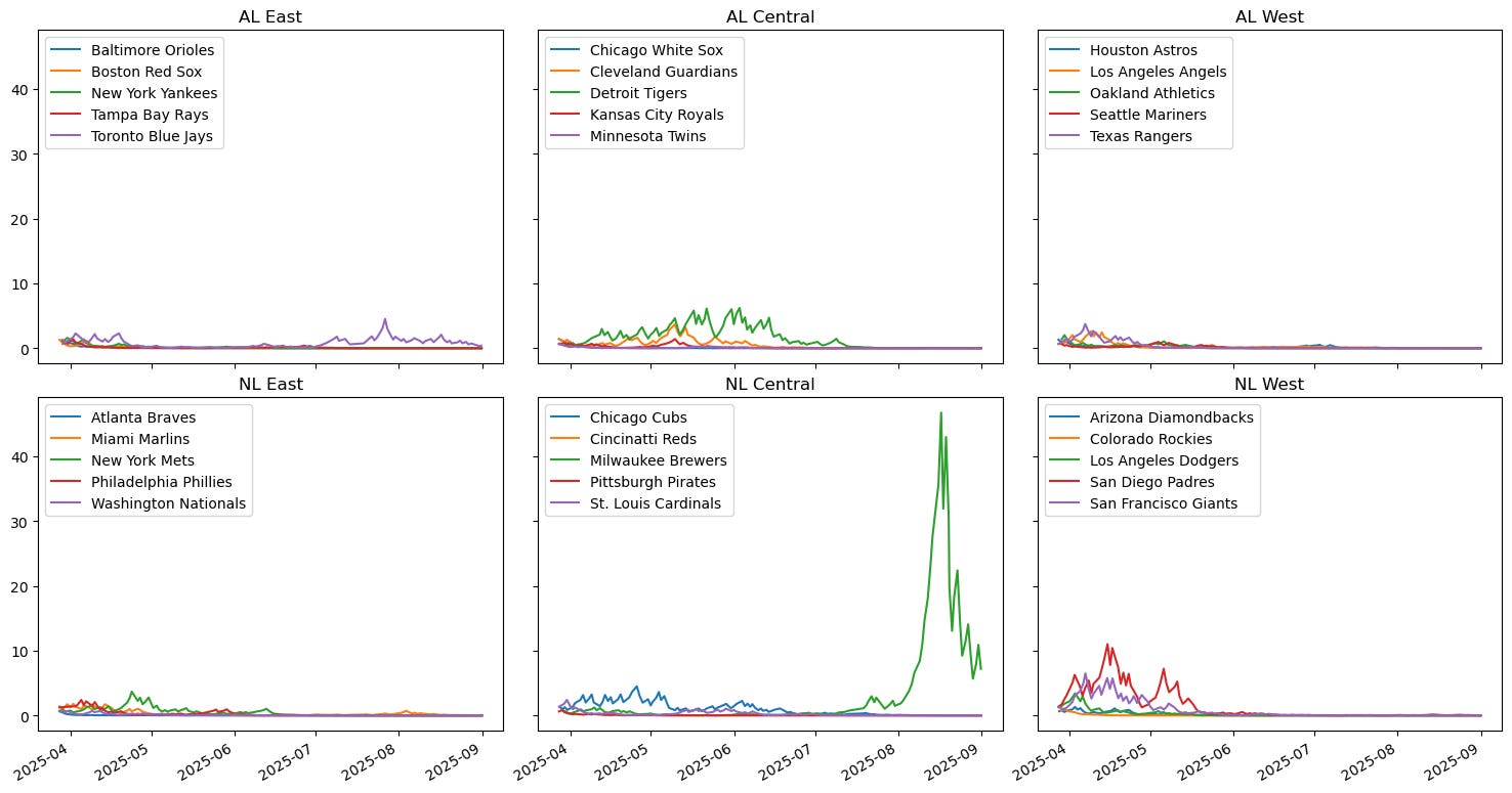
It might be fun to watch the Brewers go to the moon, but it’s less fun to have everyone else get volatility-dragged to 0 a few games in. It’s fun for a few weeks if you are a Brewers fan, but think of the ETF issuers and the fees they aren’t collecting! A more conservative value of 0.25 gives more sensible returns for 2025 and 2026:
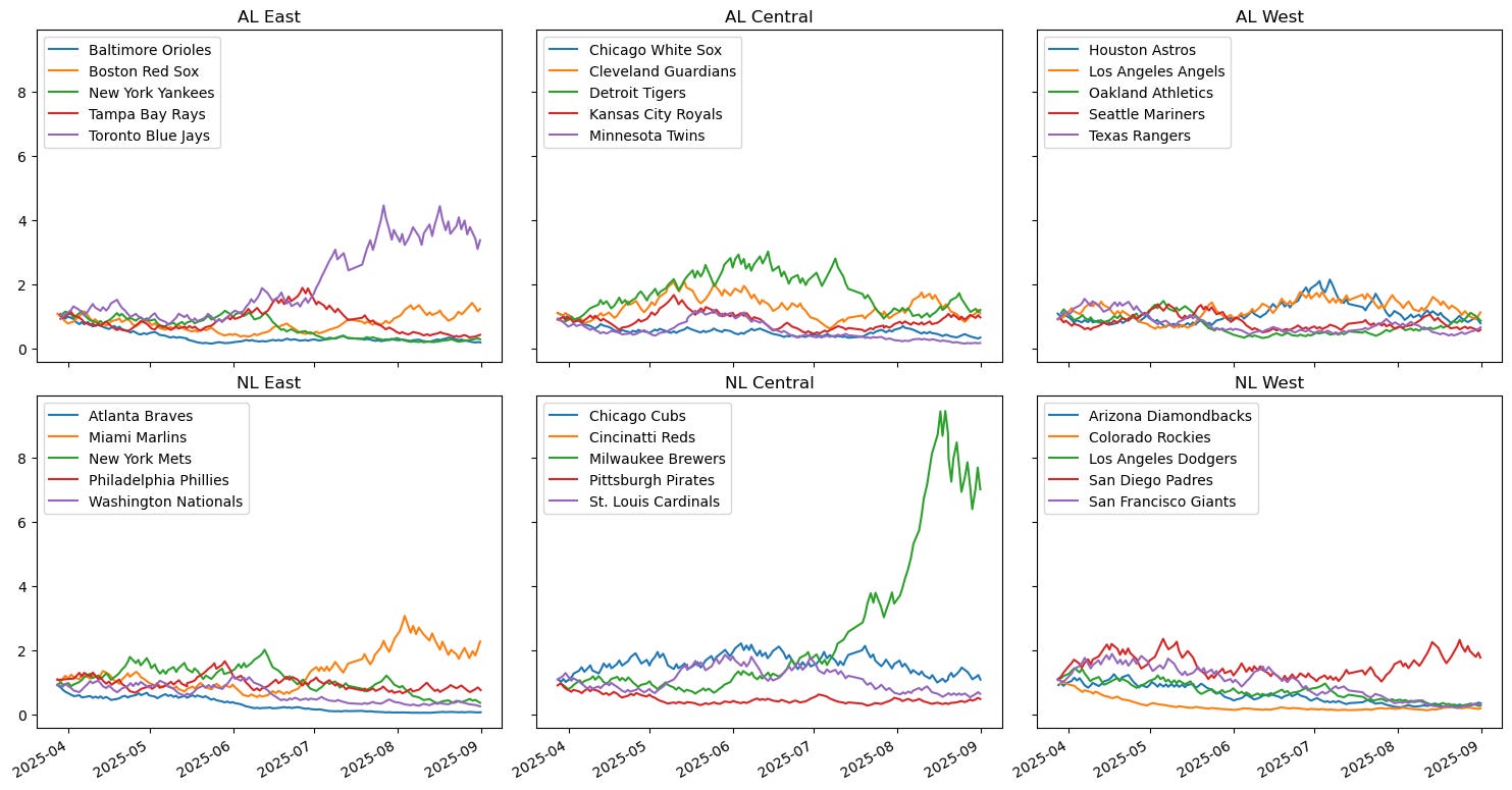
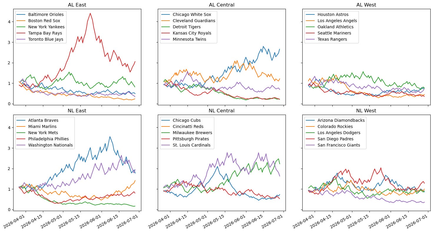
0.25 corresponds to, in a 50-50 game, putting 54.3% of AUM on the Mets and the remainder on their opponents, which means one win and one loss loses the ETF 0.75%.
So here it is in a sentence:
The ETF has the same beliefs as the market, except for acting like it has secret, moderately weak additional side information that the Mets will win, which it trades with Kelly sizing.
Three final observations. First, the ETF doesn’t merely replicate the league standings, which can be seen in the Dodgers losing money in both years despite playing pretty good baseball. Really, the ETF’s returns, like financial instruments’ returns generally, tracks performance relative to expectation. That is why the best performers in 2025 are the Brewers, who are the second best team in 2026 after the Pope’s own White Sox, because somehow every year they follow the pattern of:
Start the year having traded away half their team, meaning half their team is unknown guys called something like Cade Clap or Bo Gritz. People think “the Brewers did well last year, but they’ve traded away all their talent - who the hell are these new guys Cade Clap and Bo Gritz?”
Cade Clap and Bo Gritz have breakout seasons and the Brewers do better than everyone expected.
Over the winter, Cade Clap and Bo Gritz get traded to another team.
The new year starts - everyone thinks “Clap and Gritz are gone, who the hell are these new guys Benson Bog and Cleighton Cog? No way can the Brewers repeat last season’s performance.”
Clap and Gritz rack up -2 WAR for their new teams before getting sent to the minors. Benson Bog and Cleighton Cog have breakout seasons and the Brewers win the NL Central.
The cycle repeats.
That’s why I’m buying the Brewers ETF. And the worst performing ETF of 2026? You guessed it - it’s the Mets, who are down 83%.
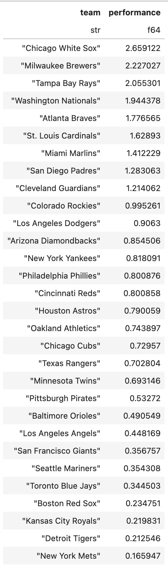
If you take the mean of these, you get baseball is down 5.4% year to date.
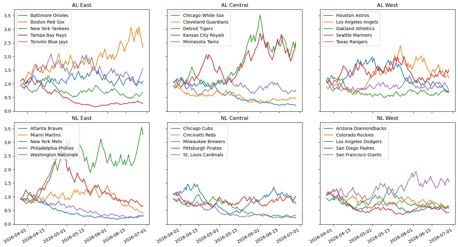
Second, there’s no rule that the ETF has to have a positive amount of bits. That is, you could have an ETF that always bets against the Mets/acts like it has side information that the Mets will lose/you get the gist by now. Here are what the -0.25 bit ETFs look like for 2026:
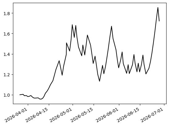
Third, the really fun part: the +0.25 ETF and the -0.25 ETF for the same team don’t have their returns sum to 0. This is clear if you remember the 81-81 case from before, where the +1.0 ETF loses over 99%, and the symmetry of the situation means the -1.0 ETF must also lose the same amount. The payout comes from if the team wins a huge number of games or loses a huge number of games, it doesn’t matter which. This means if you see David Stearns making some big moves in the off season, and you think he’s either doing great or terrible things, but you don’t know which, while you know it’s nothing in between, you can buy the Mets +0.25 ETF and the Mets -0.25 ETF, which functions something like a straddle on their performance. Here is the Mets 0.25 straddle PNL for 2026:
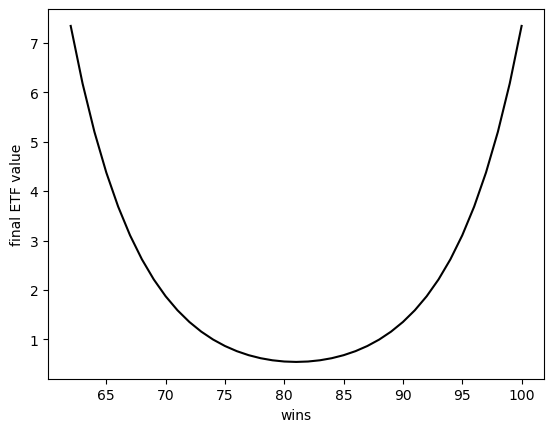
Of course, this isn’t actually a straddle, because the payoff in each ETF is exponential, not ramp function, in number of wins, so the “straddle” payoff is approximately exponential in abs(number of wins - 81). If you hate yourself and want to ruin your day, figure out the betting strategy that will give you a payout of abs(wins - 81). Assuming the market prices every game are 50-50, here is the PNL of the 0.25 “straddle” after the regular season:
This is only an approximation - there’s no liquidity on games any reasonable time out from them, so you have to place your bets right before the game, by which point people have updated their probabilities of how good the team is. But when, at the start of 2027, you find yourself thinking “who is left on this Brewers team… but hold on, this happens every year, maybe they will be excellent yet again,” your best bet might be buying the Brewers straddle.
But that’s not all - you can make far more complicated structured products. For example, if you buy the +0.25 ETF and sell the +0.35 ETF in a 2:1 ratio, here are your final payoffs:
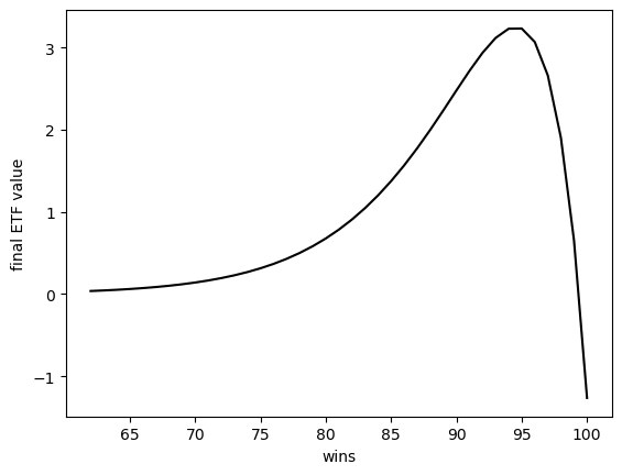
And, in fact, if you have the entire family of ETFs you can create any payoff structure you want with an unchanging ETF portfolio. That’s if you want to lose money in a really complicated way.
Appendix: the beauty and the horror of Kelly betting
Here is a rather pretty derivation of Kelly betting, which follows Cover and Thomas’ Elements of Information Theory:
There is a race with n horses. Horse k has probability p_k of winning. If horse k wins, that pays off o_k dollars for every dollar bet on that horse. (Substack doesn’t allow in-line maths, sorry.)
For each k, you are to choose b_k, which is the fraction of your bankroll you put on horse k. You have to bet your whole bankroll B on each race, although that isn’t a restriction if we assume odds are fair, because you can just place 1 / o_k on horse k for each k and perfectly preserve your bankroll.
This means if horse k wins, you now have B b_k o_k dollars.
After m races, you have B (b_{w(1)} o_{w(1)}) … (b_{w(m)} o_{w(m)}) dollars, where w(i) denotes the index of the horse that won race i.
Your average growth rate is (1 / m) \sum_{i=1}^m \log (b_{w(i)} o_{w(i)}). The log is taken because growth compounds: if we don’t take the log we get a result that, if each race adds exactly 10% to our bankroll, we don’t get an average growth rate of 10%.
Since we like money, we are trying to maximise the expected growth of our bankroll, growth being measured in log returns.
Expected growth is:
\(E(\log (b_k o_k)) = \sum_{k=1}^n p_k \log (b_k o_k)\)Algebra time. This is equal to:
\(\sum_{k=1}^n p_k \log \left(p_k \frac{b_k}{p_k} o_k\right) = \sum_{k=1}^n p_k \log p_k + \sum_{k=1}^n p_k \log \frac{b_k}{p_k} + \sum_{k=1}^n p_k \log o_k\)And now for the elegant part: using H(p) to be the entropy of p, and D(p||b) to be the KL divergence of p and b, we have
\(E(\log (b_k o_k)) = - H(p) - D(p||b) + \sum_{k=1}^n p_k \log o_k \)The only term in that which depends on b is -D(p||b). The maximum value of this is 0 at b = p. So our optimal bankroll allocation is simply if a horse has 20% probability of winning, we put 20% of our bankroll on it.
More elegant things follow. For example, define r_k = 1 / o_k, i.e., the bookmaker’s implied probability of horse k winning. Then your growth rate for Kelly betting is
That is, take the implied probabilities of your bankroll allocation and the bookmaker’s implied odds, and assess how accurate they are using KL divergence. If you are more accurate than the bookmaker, your expected growth rate is positive, and if not, it is negative. Everything is linear, and life is beautiful. But I will stop myself here.
(While I’m digressing: John Larry Kelly Jr., who came up with this Kelly system which is considered a sensible method for managing risks, died at 41 from a stroke, presumably not unrelated to his smoking six packs of cigarettes a day.)
One strange feature of this, though, is that the optimal bankroll allocation is completely independent of the payoffs o_k. There’s no mistake in the maths, but still it feels fishy. Suppose there is a fair coin which you can bet on: if it lands tails, you just get back the money you put on tails and no more, but if it lands heads, you 100x the money you put on heads. Kelly says split your money evenly between heads and tails, whereas I personally am putting more money on heads than tails. But the maths says I’m wrong!
As often happens with cases like this, the problem is one of the premises that feeds into the maths - the maths only shows my betting is only wrong assuming certain premises. (I tried to replicate Cover and Thomas’ sneaking in of the dodgy premise to make this as puzzling as possible, where they don’t ever justify why we are maximising log returns.) The problem is this: we jump from saying “we like money” to “let’s maximise expected log returns”. It seems pretty innocuous: higher log returns means more money, so clearly we want more log returns rather than less, but “we want log returns” doesn’t entail “we want to maximise expected log returns”. To illustrate: we want more money, and e^x is increasing in x, so the higher the value of e^(money) the the more money we have and so the happier we are. But it doesn’t follow that we should try to maximise expected e^(money) - that would have us taking negative expected value bets solely because they have high variance! Put simply: if we like X, it doesn’t follow that we should maximise E(X).
And look, I’m going to be honest, maximising expected log returns is really stupid. As we can see from above, this is equivalent to maximising log wealth. This captures a few intuitions about how there are diminishing returns to money and some empirical results (albeit not others) about how money relates to happiness. But a rule’s being sensible in some cases doesn’t mean it’s a good rule in general. For example, the distinction between being down 99.999% and being down 100% is trivial - you’re screwed in either case - but on the log-returns view the difference between them is infinite, and hence far larger than the difference between being down 99.999% and being up 1000% which is merely finite. I suspect Kelly sizing has stuck around because (a) the maths behind it really is quite elegant, and (b) there aren’t many good alternatives besides “maximise EV but don’t go crazy”. And if you are anything close to an EV maximiser, you are staying as far away as you can from the Mets win ETF.
Code available on GitHub.